Enhancin' our Web Scrapin'
In this post we will fix the web scraping methodology I previously used
to obtain, from OSMstats, the number of
OpenStreetMap nodes created each day, in each country. Neis Pascal, who maintains
this website, introduced last year some enhancements that broke the operation of
get_day(), a function I designed. So this time we will introduce a R
package, rvest, in order to simplify the whole process; also, we will quantify the
improvement with benchmarks.
In get_day() I used the httr package to connect to a
webpage —which in reality is a HTML document— and get its content. Objects created
by httr::content() are of xml_document class.
osmstats = "https://osmstats.neis-one.org/?item=countries&date=1-3-2021"

(httr_doc = httr::content(httr::GET(osmstats), "parsed", encoding = "UTF-8"))
## {html_document}
## <html xmlns="http://www.w3.org/1999/xhtml" lang="en">
## [1] <head>\n<title>OSMstats - Statistics of the free wiki world map</title>\n ...
## [2] <body>\n\t\n<script language="javascript">function weekendArea(axes) {var ...A xml_document is like a copy of the online page, with exactly the same
structure of tags1.
OSMstats has a page for each day —since November 1 of 2011— with the activity
for 260 territories around the world. What we want to do is extract from any page (i.e.
for any date) a tag of type <table>: a table indeed, with
the nodes created, modified, and deleted that date. The screenshot below depicts such a
table, corresponding2
to March 1 of 2021.
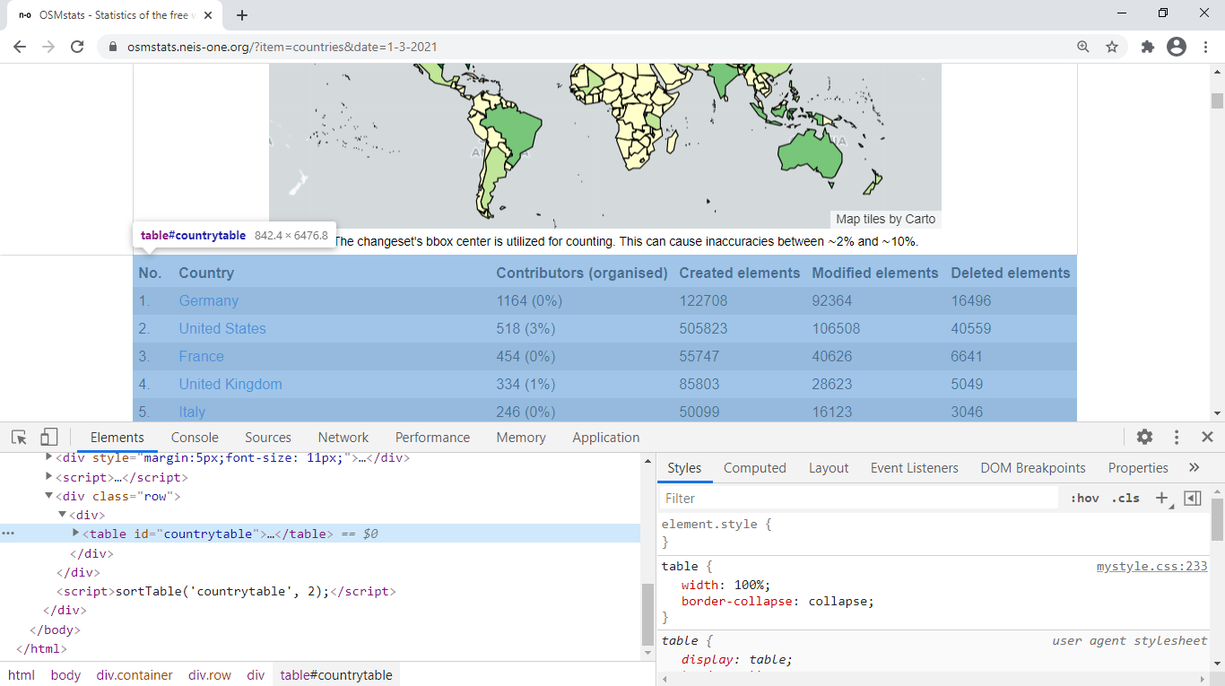
Figure 1: The <table> tag in a OSMstats webpage
Originally I had used xml2::as_list() to convert the xml_document
into a typicial R list; then, I queried the list looking for the <table>
tag, and converted each of its children into a matrix's row. These steps were
accomplished with specially designed functions:
pluck_xml = function(x) x$html$body[[12]][[14]]$div$table[-1]

row_xml = function(x) matrix(
  c( x[[2]][[1]][[1]], x[[4]][[1]], x[[6]][[1]], x[[8]][[1]], x[[10]][[1]] ), 1)
These functions can be used like this:
library(purrr)

httr_table = xml2::as_list(httr_doc) %>%
   pluck_xml() %>% map(row_xml) %>% reduce(rbind)

table_names = c("country", "contributors", "created_e", "modified_e", "deleted_e")

colnames(httr_table) = table_names; head(httr_table)
## country contributors created_e modified_e deleted_e
## [1,] "Puerto Rico" "1 (0%)" "53" "15" "2"
## [2,] "Liberia" "1 (0%)" "9464" "1695" "1852"
## [3,] "Vanuatu" "1 (0%)" "0" "4" "0"
## [4,] "Curaçao" "1 (0%)" "5" "2" "6"
## [5,] "Cape Verde" "1 (0%)" "12" "25" "1"
## [6,] "Mauritius" "1 (0%)" "0" "3" "0"If the code I've presented up to now is difficult to understand, it doesn't matter. Because
now I will show how with rvest it is possible to do the same, in an easier manner;
this package is built upon httr y xml2, so it also works with
xml_document objects. This time, we will obtain the content of the target webpage
via rvest::read_html().
library(rvest)

rvest_doc = read_html(osmstats, encoding = "UTF-8")

identical(httr_doc, rvest_doc) # documents obtained via httr and rvest seem different
## [1] FALSE## [1] TRUEOnce we get the document, we can extract the <table> with
rvest::html_node(). This function offers two options to specify the query for a tag,
and returns it as a xml_node3
object. First option is to write a CSS4
selector that precisely targets the tag we want.
Looking at the screenshot above (figure 1), the table tag
is written <table id="countrytable">; since it is the only tag
with that id in the whole page —it is the only table, by the way— we can specify the
following selector:
## # A tibble: 260 x 6
##      No. Country    `Contributors (organis~ `Created element~ `Modified element~
##    <dbl> <chr>      <chr>                               <int>              <int>
##  1     1 Puerto Ri~ 1 (0%)                                 53                 15
##  2     2 Liberia    1 (0%)                               9464               1695
##  3     3 Vanuatu    1 (0%)                                  0                  4
##  4     4 Curaçao    1 (0%)                                  5                  2
##  5     5 Cape Verde 1 (0%)                                 12                 25
##  6     6 Mauritius  1 (0%)                                  0                  3
##  7     7 Oman       1 (0%)                                  0                  3
##  8     8 Jordan     1 (0%)                                 47                 10
##  9     9 Monaco     1 (0%)                                  0                  1
## 10    10 Haiti      1 (0%)                                216                201
## # ... with 250 more rows, and 1 more variable: Deleted elements <int>
In the last code line, the extracted xml_node is inserted into
html_table() and the result is a data.frame with the OpenStreetMap
activity of the requested date. And that's it: with just three rvest functions
we have simplified the old methodology. Almost certainly, these functions have been optimized
for fast execution. Therefore, I am going to perform a benchmark to quantify
the enhancement in speed; to begin, I define a function that contains my old table
parsing method, and another one for the new one (parse_old() and
parse_rvest() respectively):
parse_rvest = function(doc) html_table(html_node(doc, "#countrytable"))[-1]

parse_old = function(doc) as_list(doc) %>% pluck_xml() %>% map(row_xml) %>%
   reduce(rbind) %>% as.data.frame() %>% set_names(table_names) %>%
   mutate(across(ends_with("_e"), as.numeric))

summary(parse_rvest(rvest_doc) == parse_old(rvest_doc)) # identical tables generated
## Country Contributors (organised) Created elements Modified elements
## Mode:logical Mode:logical Mode:logical Mode:logical
## TRUE:260 TRUE:260 TRUE:260 TRUE:260
## Deleted elements
## Mode:logical
## TRUE:260Next, I put both functions inside microbenchmark():
library(microbenchmark)

(parsing_bmark = microbenchmark(parse_rvest(rvest_doc), parse_old(rvest_doc)))
## Unit: milliseconds
## expr min lq mean median uq max neval
## parse_rvest(rvest_doc) 158.4 168.6 173.4 173.4 177.7 188.5 100
## parse_old(rvest_doc) 326.2 354.8 368.2 366.0 377.8 442.6 100boxplot(filter(parsing_bmark, time < 4.5e8),
main = "Table parsing benchmark",
ylab = "Milliseconds")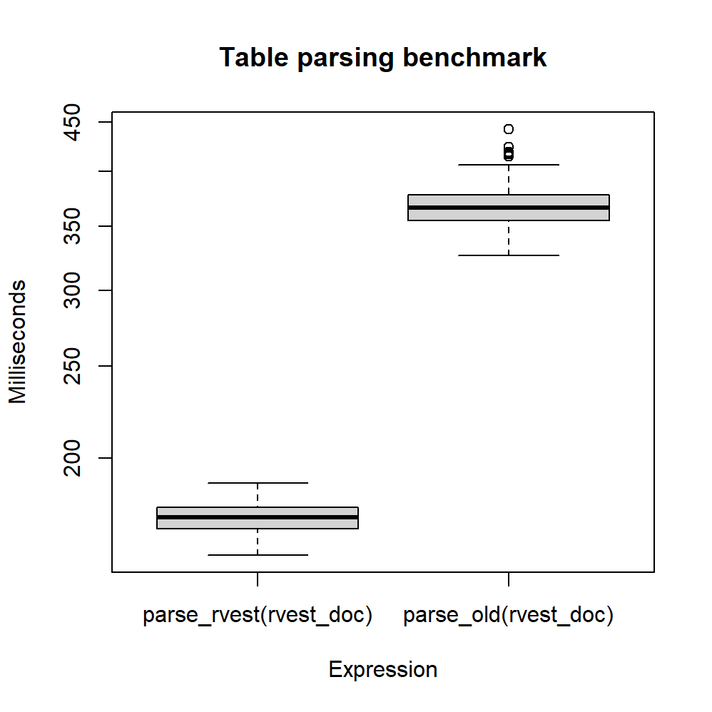
Figure 2: Benchmark of the two table parsing methods
It is clear that the new method is significantly faster, as the median execution time was
halved (from 0.37 to 0.17 seconds). Hence, from now on, I will be using rvest
whenever web scraping is required. There's still room for improvement, though. I
mentioned html_node() has two options to specify what node should be extracted.
The second option is to write a XPath
expression, which more or less works like a file's path inside a file system.
I am going to compare the extraction speed when using the same CSS selector
as before, and two XPaths. The expression "//table" means “look for a table
(remember, there is only one in each OSMstats page), no matter where it is”; let's say
this is the “easy” expression. With the other XPath I will specify in an exact manner
where is the table, much like I did with pluck_xml() in the old method; in
theory, this will be the fastest expression.
easy_css = function(doc) html_node(doc, css = "#countrytable")

easy_xpath = function(doc) html_node(doc, xpath = "//table")

exact_xpath = function(doc) html_node(doc, xpath = "body/div[3]/div[4]/div/table")

extraction_bmark = microbenchmark(easy_css(rvest_doc),
                                  easy_xpath(rvest_doc),
                                  exact_xpath(rvest_doc))

boxplot(filter(extraction_bmark, time < 4.5e6),
        main = "Table extraction benchmark",
        ylab = "Microseconds")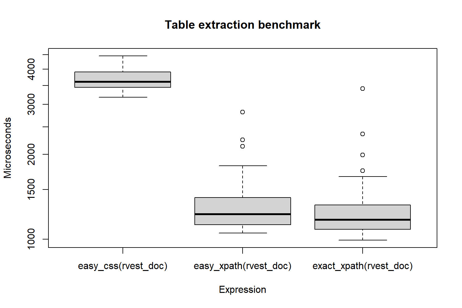
Figure 3: Benchmark of the three table extraction methods
The result is that extracting is about 2 milliseconds slower with the selector.
With the exact XPath expression there is a little improvement, but it is in the order of
microseconds. As a conclusion, in the future —when I need to obtain the daily created
OpenStreetMap elements again— I will apply the "//table" expression, which is
both fast and easy to understand.
Tags are the nodes or elements that make up a HTML document, like
<a>or<tr>.↩︎In reality, in the Countries tab of OSMstats, each page shows data corresponding to the previous day; therefore, in this example, the data is actually from February 28.↩︎
There is also
rvest::html_nodes()that can extract many tags at once, and returns axml_nodeset.↩︎Selectors are rules to select tags and apply styles in a HTML document, like
a:hover { }otr.odd { }.↩︎